Quickstart

import matplotlib.pyplot as plt
import numpy as np
import bdms

Birth, death, and mutation processes

We define a simple binary process.

birth = bdms.poisson.DiscreteProcess([1.0, 2.0])
death = bdms.poisson.ConstantProcess(1.0)
mutation = bdms.poisson.ConstantProcess(1.0)
mutator = bdms.mutators.DiscreteMutator((0, 1), np.array([[0, 1], [1, 0]]))

Simulation

Initialize random number generator

rng = np.random.default_rng(seed=0)

Initialize a tree with a root node in state 0

tree = bdms.Tree(state=0)

Simulate for a specified time

time_to_sampling = 5.0

tree.evolve(
    time_to_sampling,
    birth_process=birth,
    death_process=death,
    mutation_process=mutation,
    mutator=mutator,
    seed=rng,
)

Randomly sample survivor tips

tree.sample_survivors(p=0.5, seed=rng)

Visualization

Define keyword arguments that we’ll use repeatedly for tree visualization

viz_kwargs = dict(
    color_map={0: "red", 1: "blue"},
    h=5,
    units="in",
)

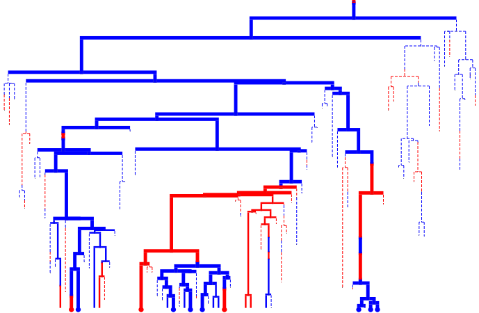
Render the full simulated tree

tree.render("%%inline", **viz_kwargs)

Partially observed trees

Prune the tree to only include the ancestry of the sampled leaves

tree.prune_unsampled()

tree.render("%%inline", **viz_kwargs)

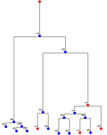
Also remove the mutation event unifurcations

tree.remove_mutation_events()

tree.render("%%inline", **viz_kwargs)

Inhomogeneous processes

We subclass the abstract class bdms.poisson.InhomogeneousProcess. To concretize, we must override its abstract method bdms.poisson.InhomogeneousProcess.λ_inhomogeneous(). We’ll use this for a death rate that linearly increases over time, and is independent of state.

class RampingProcess(bdms.poisson.InhomogeneousProcess):
    def __init__(self, intercept, slope, *args, **kwargs):
        self.intercept = intercept
        self.slope = slope
        super().__init__(*args, **kwargs)

    def λ_inhomogeneous(self, x, t):
        return self.intercept + self.slope * t

death = RampingProcess(1.0, 0.06)

Initialize tree as before

tree = bdms.Tree()
tree.state = 0

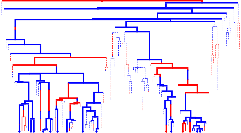
Simulate, sample, and visualize

tree.evolve(
    time_to_sampling,
    birth_process=birth,
    death_process=death,
    mutation_process=mutation,
    mutator=mutator,
    seed=rng,
)
tree.sample_survivors(p=0.5, seed=rng)
tree.render("%%inline", **viz_kwargs)

Prune and visualize

tree.prune_unsampled()
tree.render("%%inline", **viz_kwargs)

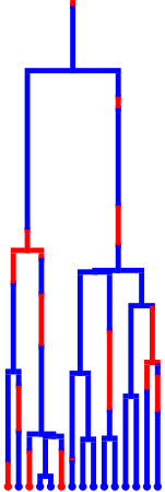
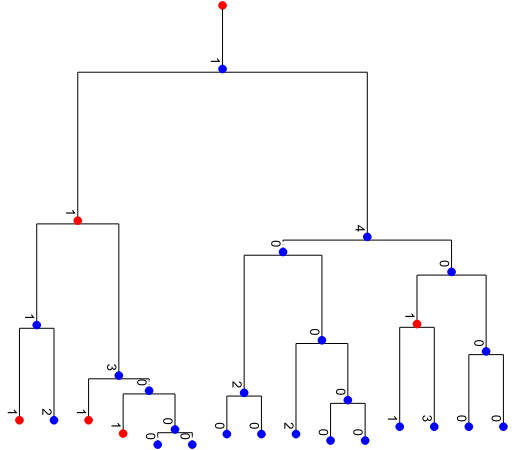
tree.remove_mutation_events()
tree.render("%%inline", **viz_kwargs)

Population size limits

Tree.evolve limits the population to capacity individuals, 1000 by default, and capacity_method sets what happens at the limit. By default (capacity_method=None), exceeding the limit is an error. We’ll use a population that roughly doubles in each unit of time, with a capacity of 100:

birth = bdms.poisson.ConstantProcess(2.0)
death = bdms.poisson.ConstantProcess(1.0)
capacity = 100

tree = bdms.Tree()
try:
    tree.evolve(
        10.0, birth_process=birth, death_process=death, capacity=capacity, seed=2
    )
except bdms.TreeError as error:
    print(error)

capacity=100 exceeded at time=2.8617821374290355

The other methods let the simulation continue:

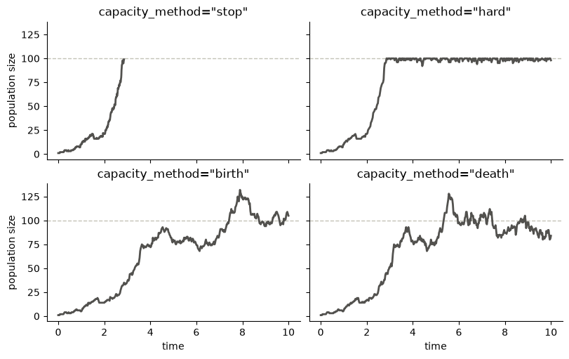
• "stop" ends the simulation when the population reaches capacity.

• "hard" kills a random individual whenever the population exceeds capacity.

• "birth" lowers birth rates as the population grows, so that births balance deaths at capacity.

• "death" raises death rates as the population grows, so that deaths balance births at capacity.

The "birth" and "death" methods need a positive death rate: without deaths, "birth" stops all births, and "death" can’t limit the population.

We simulate with each method and plot the population size over time (the dashed line is capacity). Tree.slice(t) returns the states of the lineages alive at time t, so its length is the population size:

fig, axes = plt.subplots(
    2, 2, figsize=(8, 5), sharex=True, sharey=True, layout="constrained"
)
for ax, capacity_method in zip(axes.flat, ("stop", "hard", "birth", "death")):
    tree = bdms.Tree()
    tree.evolve(
        10.0,
        birth_process=birth,
        death_process=death,
        capacity=capacity,
        capacity_method=capacity_method,
        seed=2,
    )
    end_time = max(leaf.t for leaf in tree)
    times = np.linspace(0, end_time, 400)
    population = [len(tree.slice(t, attr="state")) for t in times]
    ax.plot(times, population, color="#52514e", lw=2)
    ax.axhline(capacity, color="#c3c2b7", lw=1, ls="--", zorder=0)
    ax.set_title(f'capacity_method="{capacity_method}"')
    ax.spines[["top", "right"]].set_visible(False)
for ax in axes[1]:
    ax.set_xlabel("time")
for ax in axes[:, 0]:
    ax.set_ylabel("population size")
plt.show()